Can Tabular models be optimized by sorting the fact tables?

In multidimensional cubes you can create faster cubes by sorting your facts before you process the cube. By doing this your models will be more compressed (smaller) and your queries will run faster.

Today I wanted to test the same in Tabular. So I created 2 models with one fact table and a few dimensions. The only difference between the models are the fact table. In the first model I used the orginal table (FactInternetSales). And in the other model I used a view against FactInternetSales with a order by on all columns.

These are the tables I used

model

Then I processed and deployed the models

When checking the size of the folders that contains the fact data I was kind of surprised. I looked to be the opposite! The folder for the regular table was actually smaller than the one that represents the view. So the table seemed to be more compressed than the view.

What to you think? Is this caused by the fact that one of the facts is a table and the other one is a view? Or is the fact allready sorted in the table?

Testing row level security in Tabular (DAX)

In this post I will demonstrate how to add row level security in your tabular model. This can be a useful feature if you want to restrict access to different dimension members for different users.

First of all we need to create a new windows user on your PC / server. Lets call this user “TestUser2”

Then I will create a new table with user names and which customers they should be able of viewing.


use [AdventureWorksDW2012]

create table [UserAccess] 
(
	FullDomainUserName varchar(200),
	DomainUser varchar (100),
	CustomerKey int
)

insert into [UserAccess] values ('yourdomain\TestUser2', 'TestUser2', 11511)
insert into [UserAccess] values ('yourdomain\TestUser2', 'TestUser2', 11512)

Open the Tabular model project in Visual Studio Data Tools.

Lets add this table to the model and then create a relationship to Customer and column CustomerKey. Click “Hide from client tools” on the UserAccess table.

After you have done this your model will look like this

Screenshot useraccess

Add a new role (Model -> Roles) called TestRole. Give this read permissions.

Then add this DAX to the DAX filter on the Customer table

='Customer'[CustomerKey]=LOOKUPVALUE('UserAccess'[CustomerKey], 'UserAccess'[FullDomainUserName], USERNAME(), 'UserAccess'[CustomerKey], 'Customer'[CustomerKey]) 

Role 1

Add your new Windows users to members

Role 2

Deploy your model.

Open a Excel pivot. When Connection to the SSAS server impersonate the TestUser2 user. After doing that your pivot will look like this.

Role pivot

Creating a KPI in Tabular (DAX)

In this post I will explain how to make a simple KPI in SSAS Tabular. First step is to make two calculated measure in our model. The first one will give us the sales for 01.10.2006. This will be our base measure.

KPI_SalesYesterDay:=Calculate(SUM([Sales Amount]);Filter(Date;'Date'[Date] = DATE ( 2006; 10; 01)))

The second measure defines the target value. That might look like this.

KPI_SalesComparableDay:=Calculate(SUM([Sales Amount]);Filter(Date;'Date'[Date] = DATE ( 2005; 11; 01)))

After creating these two measures you right-click on the measure “KPI_SalesYesterDay” and click “Create KPI”.

This screen will appear

KPI 1

Use the default values. Then deploy the model to the server.

If you create a new Excel pivot it will appear like this:

KPI 2

In a more real life example you might want to use dynamic dates. Like this

KPI_SalesYesterDay:=Calculate(SUM([Sales Amount]);Filter('Date';FORMAT('Date'[Date]; "yyyy-MM-dd") = FORMAT(NOW() - 1; "yyyy-MM-dd")))

This will give us the sales for yesterday. And then subtract 365 days on the target measure to get the comparable day.

KPI_SalesComparableDay:=Calculate(SUM([Sales Amount]);Filter('Date';FORMAT('Date'[Date]; "yyyy-MM-dd") = 
FORMAT(NOW() - 365; "yyyy-MM-dd")))

Or just leave the date filtering to whatever the user chooses

Percent of total in a hierarchy (DAX)

Getting percent of total in a hierarchy is easy in DAX. In this example we will use the Geography hierarchy.

Geography 1

Then I will create 2 calculated measures in my model.

TotalSales2:=calculate(SUM([Order Quantity]);ALL('Geography'))

And

Ratio To Total:=Sum([Order Quantity]) / [TotalSales2]

The last one should be formatted as percent.

Then process and deploy your model.

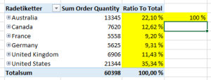
If you open an Excel pivot you should see something like this

Hierarchy Excel 2

If you summarize “Ratio To Total” in this pivot you will get 100 %.

When changing the pivot to show city instead of country the percent still works as intended.

Hierarchy Excel 3

I did not show all the cities in the screenshot above

Percent of parent in hierarchy (DAX)

Getting percent of parent in a dimension without a hierarchy is quite simple. But to get percent of parent in a hierarchy with several levels you will have to add some more code. In the current version of DAX you will have to write code for each level.

My sample query will only work for the hierarchy in the “Geography” dimension called “Geography”.

Geography 1

Then I will add 2 calculated measures to my model.

ParentSalesEmployee :=
IF (
    ISFILTERED ( 'Geography'[City] );
    CALCULATE (
        SUM ( [Order Quantity] );
        ALL ( 'Geography'[City] )
    );
    IF (
        ISFILTERED ( 'Geography'[State Province Name] );
        CALCULATE (
            SUM ( [Order Quantity] );
            ALL ( 'Geography'[State Province Name] )
        );
        CALCULATE (
            SUM ( [Order Quantity] );
            ALL ( 'Geography'[Country Region Name] )
        )
    )
)

And then

Ratio To Parent:=Sum([Order Quantity]) / [ParentSalesEmployee]

And the result will looks like this:

Geography 2

I hope hierachy handling will become better in next version of DAX…

Get number of days since last sales in DAX

Today I want to show you an sample on how to count the number of days since last sales. And the number of days between first sale and last sale.

The code is quite easy to understand

DEFINE
    MEASURE 'Internet Sales'[First order date] =
        CALCULATE ( MIN ( 'Internet Sales'[Order Date] ) )
    MEASURE 'Internet Sales'[Last order date] =
        CALCULATE ( MAX ( 'Internet Sales'[Order Date] ) )
EVALUATE
 (
    FILTER (
        SUMMARIZE (
            'Geography',
            'Geography'[City],
            "First order", 'Internet Sales'[First order date],
            "Last order", 'Internet Sales'[Last order date],
            "Days between", 1 * 'Internet Sales'[Last order date]
                - 'Internet Sales'[First order date],
            "Days since last order", 1 * TODAY ()
                - 'Internet Sales'[Last order date],
            "Sales", FORMAT (
                'Internet Sales'[Internet Total Sales],
                "Currency"
            )
        ),
        'Internet Sales'[Internet Total Sales] <> 0
    )
)
ORDER BY 'Internet Sales'[Last order date] DESC

And the result will look like this

Count days 1

A geek will always think; “how can I make this query run faster?”

One thing is to replace summarize with addcolumns. As in the sample below.

DEFINE
    MEASURE 'Internet Sales'[First order date] =
        CALCULATE ( MIN ( 'Internet Sales'[Order Date] ) )
    MEASURE 'Internet Sales'[Last order date] =
        CALCULATE ( MAX ( 'Internet Sales'[Order Date] ) )
EVALUATE
 (
    FILTER (
        ADDCOLUMNS (
            VALUES ( 'Geography'[City] ),
            "First order", 'Internet Sales'[First order date],
            "Last order", 'Internet Sales'[Last order date],
            "Days between", 1 * 'Internet Sales'[Last order date]
                - 'Internet Sales'[First order date],
            "Days since last order", 1 * TODAY ()
                - 'Internet Sales'[Last order date],
            "Sales", FORMAT (
                'Internet Sales'[Internet Total Sales],
                "Currency"
            )
        ),
        'Internet Sales'[Internet Total Sales] <> 0
    )
)
ORDER BY 'Internet Sales'[Last order date] DESC

If you check the execution time in SQL Server Profiler you will see that query 2 runs faster than query 1.

Hierarchy testing in DAX (attempt number 2)

Here is some new query samples on how DAX hierarchies work. And this time it will work 🙂

Id did a little modification of the model. I had to make a new hierachy in the employee table.

Hierachy in tabular model

Then you will have to deploy the model to the server.

My sample query looks like this:

DEFINE
    MEASURE 'Employee'[Employeelevel] =
        PATHLENGTH (
            PATH ( Employee[EmployeeKey], Employee[ParentEmployeeKey] )
        )
    MEASURE 'Employee'[ParentEmployee] =
        LOOKUPVALUE (
            'Employee'[Last Name],
            'Employee'[EmployeeKey], PATHITEMREVERSE (
                PATH (
                    'Employee'[EmployeeKey],
                    'Employee'[ParentEmployeeKey]
                ),
                2,
                1
            )
        )
    MEASURE 'Employee'[PathReverse] =
        PATHITEMREVERSE (
            PATH (
                'Employee'[EmployeeKey],
                'Employee'[ParentEmployeeKey]
            ),
            2,
            1
        )
    MEASURE 'Employee'[Path] =
        PATH (
            'Employee'[EmployeeKey],
            'Employee'[ParentEmployeeKey]
        )
EVALUATE
FILTER (
    SUMMARIZE (
        'Employee',
        'Employee'[EmployeeKey],
        'Employee'[Last Name],
        "Sales", 'Reseller Sales'[Reseller Total Sales],
        "Path", 'Employee'[Path],
        "PathItemReverse", 'Employee'[PathReverse],
        "Employeelevel", 'Employee'[Employeelevel],
        "ParentEmployee", 'Employee'[ParentEmployee]
    ),
    ISBLANK ( 'Reseller Sales'[Reseller Total Sales] ) = FALSE
)
ORDER BY 'Employee'[ParentEmployee], 'Employee'[EmployeeKey]

And the result looks like this

hierarchy correct

To verify the result I made an Excel pivot.

How to use “CrossJoin” in DAX

The “CrossJoin” function returns the Cartesian product of all rows from all tables in the arguments. In my sample below I want to have sales per year per city.

EVALUATE
ADDCOLUMNS (
SUMMARIZE (
CROSSJOIN (
VALUES ( 'Date'[Calendar Year] ),
VALUES ( Geography[City] )
),
'Date'[Calendar Year],
Geography[City]
),
"Sum of Sales", CALCULATE ( SUM ( 'Internet Sales'[Sales Amount] ) )
)

And the result looks like this

CrossJoin1

But as you can see I get a lot of empty rows. To remove these empty rows I add a filter to my query. I also moved my calculation outside the main query to make it more readable.

DEFINE
MEASURE 'Internet Sales'[Sales] =
SUM ( 'Internet Sales'[Sales Amount] )
EVALUATE
ADDCOLUMNS (
FILTER (
SUMMARIZE (
CROSSJOIN (
VALUES ( 'Date'[Calendar Year] ),
VALUES ( Geography[City] )
),
'Date'[Calendar Year],
Geography[City]
),
'Internet Sales'[Sales] <> 0
),
"Sum of Sales", 'Internet Sales'[Sales]
)

CrossJoin 1

Basic query optimalization in DAX

What can we do to make queries as fast as possible? Here is some tips 🙂

In my simple test I want to see the sales for year 2009. To make sure my queries does not hit any cache I’m clearing it using XMLA. In my first query I will try to use the ROW function and sum up the internet sales

EVALUATE
ROW (
"Sales", CALCULATE (
SUM ( 'Internet Sales'[Sales Amount] ),
'Date'[Calendar Year] = 2008
)
)

When watching the profiler I can see that this query took 156 milliseconds. The reason why this takes quite long is that we are one the row level.

Lets switch to table level.

EVALUATE
FILTER (
SUMMARIZE (
'Date',
'Date'[Calendar Year],
"Sales", SUM ( 'Internet Sales'[Sales Amount] )
),
'Date'[Calendar Year] = 2008
)

This query took 78 milliseconds. Twice as fast as the first query.

What if I move the calculation using ADDCOLUMNS outside the SUMMARIZE?

EVALUATE
ADDCOLUMNS (
FILTER (
SUMMARIZE ( 'Date', 'Date'[Calendar Year] ),
'Date'[Calendar Year] = 2008
),
"Sales", CALCULATE ( SUM ( 'Internet Sales'[Sales Amount] ) )
)

This query took 62 milliseconds

Do you have an even better optimalization tip? Feel free to drop me an mail

Comparable day in DAX

In many companies they want to compare todays sales with the comparable day last year. To find the comparable day we subtract 364 from todays date. In this sample todays date is 15 january 2007.

To see what dates we should get we can run this SQL

select '2007/01/15' as TodaysDate, DateName(dw, '2007/01/15') As 'DayName', 
dateadd(day, -364, '2007/01/15') As ComparableDay, DateName(dw, dateadd(day, -364, '2007/01/15')) As ComparableDayName

And this will return this result

Comparable day 3

To check the values for these dates we can run these DAX queries

EVALUATE
FILTER (
    ADDCOLUMNS (
	VALUES ('Date'[Date]),
        "Sales this day", 'Internet Sales'[Internet Total Sales]
    ),
    'Date'[Date] = DATE ( 2007, 01, 15 )
)

EVALUATE
FILTER (
    ADDCOLUMNS (
	VALUES ('Date'[Date]),
        "Sales this day", 'Internet Sales'[Internet Total Sales]
    ),
    'Date'[Date] = DATE ( 2006, 01, 16 )
)

The final query where we put all together looks like this

EVALUATE
FILTER (
    ADDCOLUMNS (
        VALUES ( 'Date'[Date] ),
        "Comparable day", CALCULATE (
            'Internet Sales'[Internet Total Sales],
            DATEADD ( 'Date'[Date] , -364, Day)
        ),
        "Sales this day", 'Internet Sales'[Internet Total Sales]
    ),
    'Date'[Date] = DATE ( 2007, 01, 15 )
)

Comparable day 4

Please note that this sample requires a date dimension that has the date 2006/01/16. If you are unsure about this you will have to change the query. The -364 approach will have issues if last year was a leap years.